Forecasting Asset Prices Using VAR and Granger Causality

Forecasting Gold and Oil has garnered major attention from academics, investors and Government agencies alike. These two products are known for their substantial influence on the global economy. However, what is the relationship between these two assets? What generally happens to Gold prices when Oil takes a plunge? We can use a statistical technique known as Granger Causality to test the relationships of Gold, Oil, and some other variables. We can also use a VAR model to forecast the future Gold & Oil prices.
Exploratory Analysis
Let’s load the data and conduct some analysis with visualizations to understand more of the data. Exploratory data analysis is quite extensive in multivariate time series. I will cover some areas here to get insights into the data. However, it is advisable to conduct all statistical tests to ensure our clear understanding of data distribution.
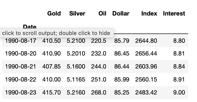
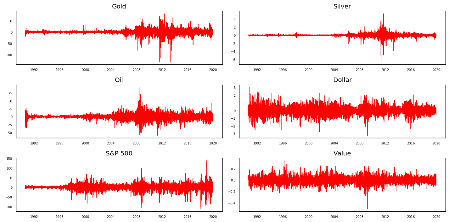
In our dataset, we have six variables: Gold, Silver, Oil, US Dollar, Interest, and a Stock Market Index. The stock market index we’ve used was the Dow Jones Industrial Average. We usually use linear regression to determine if there is a correlation between specific variables. Instead, we’re going to determine if any of these variables directly causes movement in the other variables.
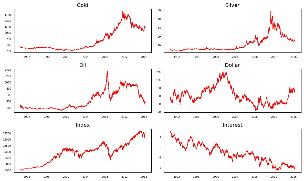
Here, we can see different trends for six of our variables. It would be helpful if we established whether or not our time series followed a normal (or Gaussian) distribution. We will do this based on the test for normality based on the Jarque-Bera test.
Jarque-Bera Test
There are actually three test that we could have implemented for testing normality; however, we will focus on just one: the Jarque-Bera Test.
The Jarque-Bera goodness-of-fit test determines whether a sample data have the skewness and kurtosis matching a normal distribution.
$$k_{3}=\frac{\sum^{n}{i=1}(x{i}-\bar{x})^{3}}{ns^{3}} ,,,,,,, k_{4}=\frac{\sum^{n}{i=1}(x{i}-\bar{x})^{4}}{ns^{4}}-3 $$
$$JB = n \Bigg(\frac{(k_{3})^{2}}{6}+\frac{(k_{4})^{2}}{24}\Bigg) $$
where $x$ is each observation, $n$ is the sample size, $s$ is the standard deviation, $k_{3}$ is skewness, and $k_{4}$ is kurtosis. The null hypothesis, $H_{0}$, follows that the data is normally distributed; the alternative hypothesis, $H_{A}$, follows that the data is not normally distributed.
There is a simple script we can use in python to determine the goodness of fit, the kurtosis, and the skewness.
from scipy import stats
stat, p = stats.normaltest(df.Gold)
print('Statistics=%.3f, p=%.3f' % (stat, p))
alpha = 0.05
if p > alpha:
    print('Data looks Gaussian (fail to reject H0)')
else:
    print('Data does not look Gaussian (reject H0)')
Lets test out the goodness of fit on the Gold variable.
Statistics=818.075, p=0.000
Data does not look Gaussian (reject H0)
As we can see, we recieve a p-value and a test statistic in return. While we don’t have a Chi-Square chart to determine the critical region, we do have a p-value, which is basically zero.
A p-value less than 0.05 basically means our test statistic falls within the critical region (inside the tail); therefore, we can reject the null hypothesis. The dataset is not normally distributed, which we probably could have assumed by looking at the time series plots from before.
Lets compare kurtosis and skewness for both the Oil and Gold variables.
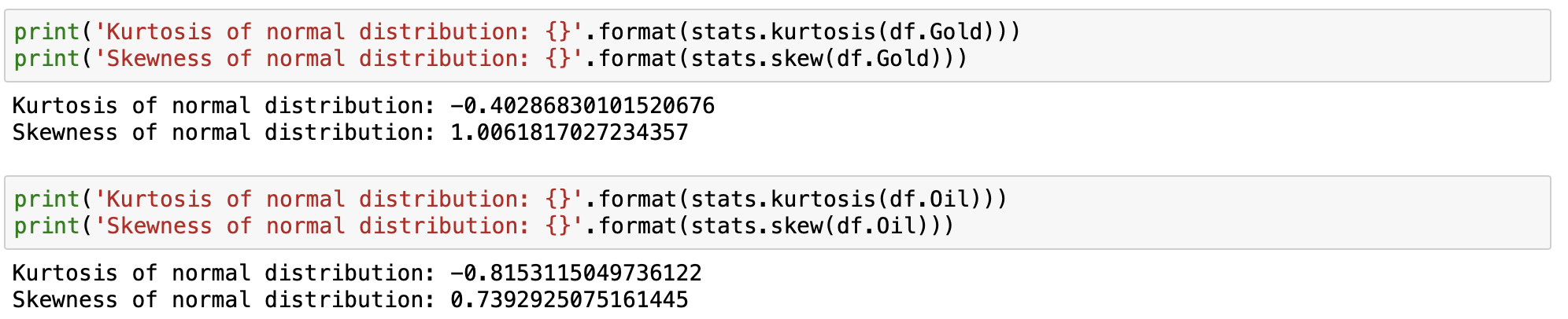
These two distributions can provide us with some intuition about the distribution of our data. A value close to 0 for kurtosis indicates a normal distribution where asymmetrical nature is signified by a value between -0.5 and +0.5 for skewness. The tails are heavier for kurtosis greater than 0 and vice versa. Moderate skewness refers to the value between -1 and -0.5 or 0.5 and 1.
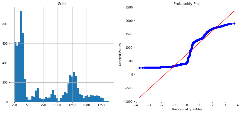
Based on the normal probability plot, we can see that the dataset is far from normally distributed.
The VAR Model
Considering that our dataset isn’t normally distributed, we can use this information to build a VAR model. The construction of the model will be based on the following steps:
- Testing for autocorrelation
- Spliting the time series into Training and Testing data sets
- Testing for Stationarity
- Testing for Causation using Granger Causality
- Conducting a forecast evaluation
Auto-Corrlation
Autocorrelation refers to how correlated a time series is with its past values as a function of the time lag between them.
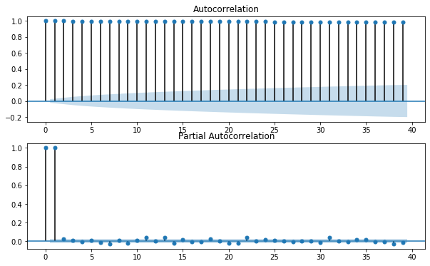
The following plot shows the autocorrelation for the Gold time series. As we can see, each value is highly correlated with the previous value. We have an autocorrelation of +1, which represents a perfect positive correlation. An increase seen in one time series leads to a proportionate increase in the other time series.
We need to apply transformation and neutralize this time series stationary. It measures the linear relationships. Even if the autocorrelation is minuscule, there may still be a nonlinear relationship between the time series and a lagged version of itself.
Spliting the time series into Training and Testing data sets
The VAR model will be fitted on X_train and then used to forecast the next 15 observations. These forecast will be compared against the actual present test data.
nobs = 15
X_train, X_test = df[0:-nobs], df[-nobs:]

#check size
print(X_train.shape)
print(X_test.shape)
Testing for Stationarity
Intuitively, stationarity implies that the statistical properties of the process are consistent. In other words, the mean, variance and autocorrelation structure do not change over time. Stationarity can be defined in precise mathematical terms, but for our purpose we mean a flat looking series, without trend, constant variance over time, a constant autocorrelation structure over time with no periodic fluctuations (seasonality).
In order to make the time series stationary, we need to apply a differencing function on the training set. However, this is an iterative process where we after first differencing, the series may still be non-stationary. We may have to apply a second difference or log transformation to standardize the series in such cases.
The following demonstrates what time series would generate with our differencing technique.
Testing Causation using Granger’s Causality Test
The question of what event caused another, or what brought about a certain change in a phenomenon, is a common one. While a naive interpretation of the problem may suggest simple approaches like equating causality with high correlation, or to infer the degree to which $x$ causes $y$ from the degree of $x$’s goodness as a predictor of $y$, the problem is much more complex. As a result, rigorous ways to approach this question were developed in several fields of science.
This can be done one of two different ways:
- Casual inference over random variables, representing different events. The most common example are two variables, each representing one alternative of an A/B test, and each with a set of samples/observations associated with it.
- Casual inference over time series data (and thus over stochastic processes). Examples include determining wehther (and to what degree) aggregate daily stock prices drive (and are driven by) daily trading volume, or causal relatioons between volumns of Pacific sardine catches, northern anchovy catches, and sea suface temperature.
Granger Casuality Test Results
Granger’s causlity tests the null hypothesis, $H_{0}$, that the coefficients of past values in the regression equation is zero. In simplier term, the past values of time series, $X$, do not cause other series, $Y$. If the p-value obtained from the test is lesser than the significance level of 0.05, then, you can safely reject the null hypothesis.
The following code was performed on the transformed dataset:
from statsmodels.tsa.stattools import grangercausalitytests

maxlag = 5
test = 'ssr_chi2test'

def granger_causation_matrix(data, variables, test='ssr_chi2test', verbose=False):
    X_train = pd.DataFrame(np.zeros((len(variables), len(variables))), columns=variables, index=variables)
    for c in X_train.columns:
        for r in X_train.index:
            test_result = grangercausalitytests(data[[r, c]], maxlag=maxlag, verbose=False)
            p_values = [round(test_result[i+1][0][test][1], 4) for i in range(maxlag)]
            if verbose:
                print(f'Y = {r}, X = {c}, P Values = {p_values}')
            min_p_value = np.min(p_values)
            X_train.loc[r, c] = min_p_value
    X_train.columns = [var + '_x' for var in variables]
    X_train.index = [var + '_y' for var in variables]
    return X_train

granger_causation_matrix(X_train, variables = X_train.columns)
The code provided the following matrix:
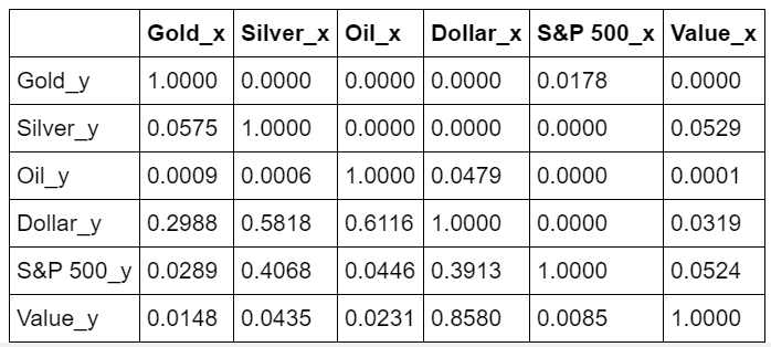
The row are the responses $Y$ and the columns are the predictors $X$.
-
If we take the value 0.0000 in (row 1, column 2), it refers to the p-value of the Granger’s Causality test for
Silver_xcausingGold_Y. The 0.0000 in row 2, column 1 refers to the p-value ofGold_ycausingSilver_x. -
As we can see,
Gold_xisn’t typically caused by any of the other variables. However, movements in the variableGold_xonly appears to be caused by the variableUSD_yThis intuitively makes sense, as the value of gold is often tied to the US Dollar and some in the investment community consider gold as a hedge against inflation (the same for the variablesSilver_xandUSD_y). -
The
Interest_xvariable only seems to cause movements inSilver_y; however,Interest_ydoes appear to cause movements in theUSD_x, which also makes sense. -
The
Index_yvariable appears to cause movements in the variablesSilver_x,Oil_x, andUSD_x.
So, looking at the p-values, we can assume that (except Oil) most of the variables (time series) in the system are interchangeably causing each other. This justifies the VAR modeling approach for this system of multi time-series to forecast.
Testing for Co-integration
Regression errors are a linear combination of two unit root series ($X$ and $Y$) of the following equation:
$$\varepsilon=Y_{t}-\alpha-\beta X_{t} $$
If $X_{t}$ and $X_{t}$ have a unit root, this usually means $\varepsilon_{t}$ also has a unit root. This is the cause of a spurious regression problem.
However, there are some cases when the unit root in $Y$ and $X$ cancel each other out and $\varepsilon_{t}$ does not have any unit root. In this special case, the spurious regression problem vanishes. This phenomenon is referred to as cointegration, which measures the equilibrium spread between two non-stationary time series measured by constant terms $\alpha$. If the error term is stationary then we can say that cointegration and an equalibrium spread exist.
For testing co-integration, we used the Johansen method to test for co-integration using the following python function:
from statsmodels.tsa.vector_ar.vecm import coint_johansen

def cointegration_test(transfrom_data, alpha=0.05):
    """Perform Johanson's Cointegration Test and Report Summary"""
    out = coint_johansen(transform_data, -1, 5)
    d = {'0.90':0, '0.95':1, '0.99':2}
    traces = out.lr1
    cvts = out.cvt[:, d[str(1-alpha)]]
    def adjust(val, length=6):
        return str(val).ljust(length)

    # Summary
    print('Name   :: Test Stat > C(95%)       => Signif   \n', '--'*20)
    for col, trace, cvt in zip(transform_data.columns, traces, cvts):
        print(adjust(col), '::', adjust(round(trace, 2), 9), ">", adjust(cvt, 8), '  =>  ', trace >cvt)


cointegration_test(X_train)
What is VAR?
Vector Autoregression (or VAR) is a multivariate forecasting algorithm that is used when two or more time series influence one another. In order to use VAR, there needs to be at least two time series for our variables and the time series needs to influence one another.
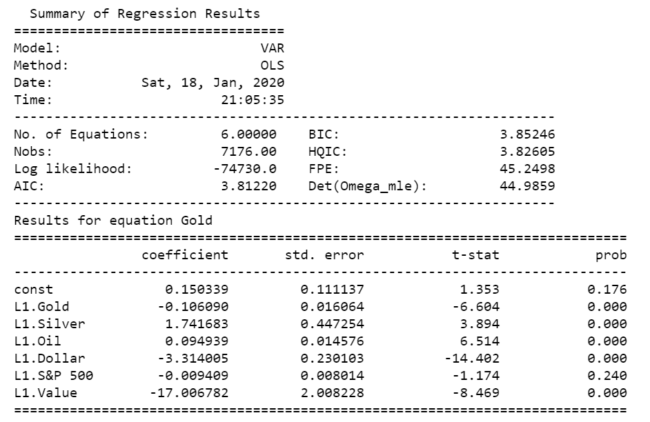
VAR is considered a ‘autoregressive’ model because each variable is modeled as a function of past values. That is, predictors are nothing but lags (time delayed values) of the series.
We’ve created models for predicting all six of our variables, which has provided the coefficients, residuals, and the AIC for the particular model. We can now begin with the forecasting.
Conducting a forecast evaluation
Now we can plot the historical observations along with the forecasted observations back to their original scale. Let us assess the differences between the two time series plots.
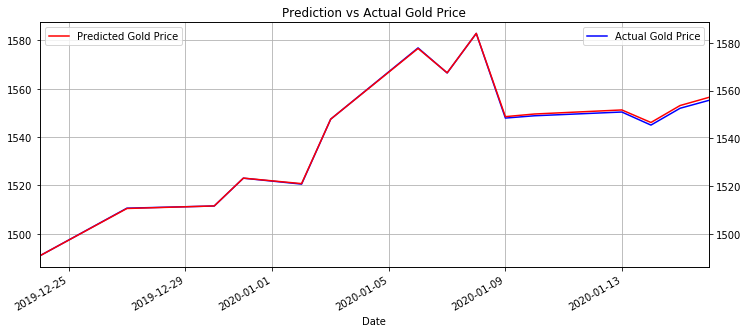
As we can see, the forecasted observations are pretty much in line with the historical observations used for forecasting Gold prices. There is a very slight deviation between the historical and forecasted observations started from Janurary 9th, however, this divergence is very slight.
Conclusion
There are many different variables that can account for the changes in different financial markets. These changes may or may not always occur in financial markets. Nonetheless, this tutorial can demonstrate how we can use the relationship in certain financial markets to create models for forecasting.
GitHub Code
Click here for the full GitHub Code and full explainations.
Andre Sealy
Quant Research / Data Scientist / Writer
My research interests involves Quantitative Finance, Mathematics, Data Science and Machine Learning.