Does Diversification Always Matter?

I’ve previously talked about Modern Portfolio Theory (MPT) and diversification, the assumptions underlying MPT, and the construction of a Portfolio Frontier (PF). When most people consider diversifying their portfolio, they consider limiting their downside risk. However, it is possible to construct a portfolio that maximizes return with the least volatility (choosing a portfolio that lies somewhere along the PF).

Now, I will further expand upon why diversification helps maximize risk-adjusted returns and express the limits of diversification.

What Makes a Portfolio?

We can define a portfolio as a combination of $N$ assets with $N$ portfolio weights that sum to unity:

$$ \begin{equation} \textbf{w}=[w_1,\ldots,w_N],\quad\sum^{N}_{n=1}w_n=1. \end{equation} $$

The weight, $w_N$, represents the proportion of the $n$th asset in the portfolio. If $M_n$ and $P_n$ are the number and price of the $n$th asset, then $w_n$ is simply the total value of the $n$th asset normalized by the value of the portfolio:

$$w_n=\frac{M_nP_n}{M_1P_1+\ldots+M_nP_N}$$

Weights can be negative, such we could short sell an asset (profiting from asset price going down). Also, weights could be greater than unity, meaning that we are using leverage. We won’t get into these complicated scenarios and use only the basic assumptions in the summary of our portfolio.

Imagine, for example, that we had an investment account of $\mathrm{$}10,000$ with $40$ shares of stock $A$ at $\mathrm{$}150$ per share, $50$ shares of stock $B$ at $\mathrm{$}20$ per share, and $25$ shares of stock $C$ at $\mathrm{$}120$ per share. Then our portfolio with weights would be

Asset	Shares	Price per share	Investments	Weight
$A$	40	150	6000	0.6
$B$	50	20	1000	0.1
$C$	25	120	3000	0.3

However, the weights need not be just the proportion of a given stock or asset. For example, suppose we were trading on margin, with $\mathrm{$}8,000$ in our account to support our $\mathrm{$}10,000$ investment. If we withdrew $\mathrm{$}2,000$ from our investment account, then our portfolio in dollars would be unchanged, but our portfolio weights would have changed:

Asset	Shares	Price per share	Investments	Weight
$A$	40	150	6000	0.6
$B$	50	20	1000	0.1
$C$	25	120	3000	0.3
Margin			-2000

The weights change because the normalizer changes from $\mathrm{$}10,000$ to $\mathrm{$}8,0000$.

Defining risk and reward

Now that we have defined what a portfolio is, we can outline what we want to do. We can construct a portfolio that maximizes reward and minimizes risk, where “reward” is defined as overal portfolio return and “risk” is defined as the volatility ($\sigma$ or $\sigma^2$) of that return.

Diversification with uncorrelated assets

We can derive the mean-variance analysis by calculating the mean (expected return) and the variance on that portfolio. Let $R_n$ denote the return on the $n$th asset in a portfolio. By definition, its mean and variance are

$$ \begin{aligned} \mathbb{E}[\mathbb{R_n}]\overset{\Delta}{=}&\mu_n,\\ \mathbb{V}[R_n]=&\mathbb{E}[(R_n-\mu_n)^2]\overset{\Delta}{=}\sigma^2_{n}.\\ \end{aligned} $$

Now let $R_p$ denote the return on the entire portfolio, this is the quantity we’re interested in. By the linearity of expectation, we have

$$ \begin{aligned} R_p\overset{\Delta}{=}&w_1R_1+\dots+w_NR_N,\\ \Downarrow & \\ \mathbb{E}[R_p]=&\mathbb{E}[w_1R_1+\dots+w_NR_N]\\ =&w_1\mathbb{E}[R_1]+\dots+w_N\mathbb{E}[R_N]\\ =&w_1\mu_1+\dots+w_N\mu_N\\ \overset{\Delta}{=}&\mu_p \end{aligned} $$

The first line of this equation is just an accounting identity. It’s how we would calculate the return on our portfolio given weights $\textbf{w}$ and returns $R_1,\ldots,R_N$. The variance of our portfolio’s return is

$$ \begin{aligned} \mathbb{V}[R_p]&=\mathbb{E}[(R_p-\mu_p)^2]\\ &=\mathbb{E}\Big[\big((w_1R_1+\dots+w_NR_N)-(w_1\mu_1+\dots+w_N\mu_N)\big)^2\Big]\\ &=\mathbb{E}\Big[\big((w_1(R_1-\mu_1)+\dots+w_n(R_N-\mu_N)\big)^2\Big]\\ &\overset{\Delta}{=}\sigma^2_p. \end{aligned} $$

If we have $N$ assets in our portfolio, and we square the term in the last line in this equation, we get $N^2$ terms inside this expectation. We can write the variance for a single combination $R_n$ and $R_m$ as:

$$ \begin{aligned} \mathbb{E}[w_nw_m(R_n-\mu_n)(R_m-\mu_m)]&=w_nw_m\mathbb{E}[(R_n-\mu)(R_m-\mu)]\\ &=w_nw_m\text{Cov}[R_n,R_m]\\ &=w_nw_m\sigma_{nm}\\ &=w_nw_m\sigma_n\sigma_m\rho_{nm}, \end{aligned} $$

where $\sigma_{nm}$ and $\rho_{nm}$ are the covariance and correlation between the $n$th and $m$th assets respectively. This provides some basic definitions from probability. Recard that

$$ \rho_{mn}=\frac{\text{Cov}[R_n, R_m]}{\sigma_n\sigma_m}. $$

Here’s the main point: The variance of our portfolio is a function of the covariances between the assets in the portfolio. We can represent this compactly using a covariance matrix:

$$ \begin{bmatrix} w_1^2\sigma_1^2 & \dots &w_1w_N\sigma_{1N}\\ \vdots & \ddots & \vdots \\ w_Nw_1\sigma_{N1} & \dots & w^2_N\sigma^2_N\\ \end{bmatrix}=\textbf{w}^T \begin{bmatrix} \sigma^2_1 & \dots & \sigma_{1N} \\ \vdots & \ddots & \vdots \\ \sigma_{N1} & \dots & \sigma^2_{N} \\ \end{bmatrix}\textbf{w} $$

Notice that there are $N$ variance terms (the diagonal of the covariance matrix), while there are $N^2-N$ covariance terms (everything else in the matrix). This means that the correlations between assets control our portfolio’s volatility. Positive or negative correlation between asset controls our portfolio’s volatility. Positive or negative correlation between assets can increase portfolio volatility, while uncorrelated assets decrease volatility.

So what exactly is “Diversification?” According to Fidelity, it’s simply “spreading your investments around so that your exposure to any one type of asset is limited.” However, we’ve learned that it’s much more nuanced than that.

As far as Modern Portfolio Theory, diversification is selecting uncorrelated assets, thereby reducing the variance of our portfolio’s returns. Failing to be diversified doesn’t necessarily mean owning just a small number of assets. In theory, we would own many highly correlated assets, which would increase the variance in our expected returns (which is different from what we want).

Mean-variance analysis

Now that we better understand diversification, we can start talking about a mean-variance framework. Let’s assume that, all things equal, investors prefer higher expected returns and lower volatility. We believe investors only care about the return on their entire portfolio rather than on a single asset. In other words, we care about $R_p$, not any individual $R_n$. Given the observed or assumed expected returns and covariance between assets, what portfolios should we prefer?

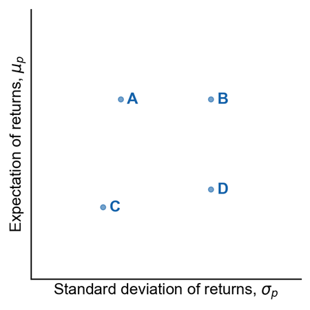
Considering the following image. On the $x$-axis is the standard deviation of a portfolio’s return $\sigma_p$, and the $y$-axis is the expected return $\mu_p$. This is call the risk-return spectrum.

Considering our assumptions, an investor should prefer portfolio $B$ over $D$, since both have the same volatility but $B$ has higher expected returns. Broadly speaking, investors want to be in the top-left corner: a portfolio with the maximum return possible with the smallest amount of risk.

How do we find the weights that will allow this to happen? Imagine we have a fixed set of assets (considering there are only so many assets we can own). We can estimate returns, variances, and covariances however we’d like, for example, by looking at historical data. Now let $\Sigma$ denote the covariance matrix, and let $\textbf{r}$ be an $N-vector$ of expected returns, i.e. $\textbf{r}\overset{\Delta}{=}[\mu_1,\ldots,\mu_N]$. Then the mean-variance portfolio optimization problem is:

$$ \begin{aligned} \underset{\textbf{w}}{\min}&\quad\textbf{w}^T\Sigma\textbf{w},\\ \text{subject to}&\quad \textbf{w}^T\textbf{r}=K,\\ \text{and}&\quad\sum_nw_n=1, \end{aligned} $$

where $K$ is a user specified hyperparameter that controls the desired expected return. In other words, w want to minimize the variance/covariance terms while ensuring our weights normalize to unity and gives us our expected portfolio return $K$ given our estimated expected asset returns $\textbf{r}$.

The two asset example

Let’s consider the special case of two assets, stock $A$ with weight $w_1$ and stock $B$ with weight $w_2$. This will allow us to carefully reason about what is happening. Since $w_1+w_2=1$, we can easily visualize all possible portfolio by sweeping $w_1\in[0,1]$, calculating $w_2\overset{\Delta}{=}1-w_1$, and then computing the $(x,y)$-coordinates in the risk-reward spectrum:

$$ \begin{aligned} &\mathbb{E}[R_p]=w_1\mu_2+w_1\mu_2, \\ &\mathbb{V}[R_p]=w^2_1\sigma^2_1+w^2_2\sigma^2_2+2w_1w_2\sigma_1\sigma_2\rho_{12} \end{aligned} $$

Suppose that stock $A$ had an average monthly return of 2 and a standard deviation of 10, while stock $B$ had an average return of $1$ and a standard deviation of $6$. Suppose their correlation if $0.35$. How would a portfolio of two stocks perform? We can construct a table comparing expected portfolio return and volatility for a variety of different weights $\textbf{w}$.

$w_1$	$w_2$	$\mu_p$	$\sigma$
$0$	$1$	$1.00$	$6.00$
$0.25$	$0.75$	$1.25$	$5.86$
$0.5$	$0.5$	$1.50$	$6.67$
$0.75$	$0.25$	$1.75$	$8.15$
$1$	$0$	$2.00$	$10.00$
$1.25$	$-0.25$	$2.25$	$12.06$

This table shows the potential combination of weights we could have for our two assets. Instead of taking $100%$ of stock $A$ and $100%$ of stock $B$, we would take a combination of the two. Portfolio Theory doesn’t tell us which combination we should take; that would depend on where you want to be on the risk-reward spectrum.

We could adopt a portfolio $100%$ of stock A for the maximum return, which is very risky. We could adopt a portfolio $25%$ of stock $A$ and $75%$ of stock $B$ for the least amount of volatility. We could also short stock $B$ to go beyond the maximum return, which will greater increase or risk.

Plotting all the possible portfolios for these two stocks gives us the following image. Obviously, the relationship between risk and reward is nonlinear, as the portfolio is a functional relationship betweeen $\mu_p$ $\sigma_p$. As mentioned before, this is known as an efficient frontier or portfolio frontier.

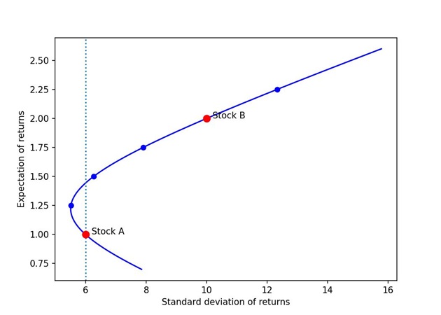
Now we can see the risk-returns of holding just stock $A$ or just stock $B$. Clearly just holding stock $A$ is less risky than holding just stock $B$. However, notice that if we draw a vertical line straight up from stock $A$, we intersect the curve. This tells us that with a creative selection of portfolio weights, we can get the same risk but with a higher expected return.

So it’s rational to prefer this point over just stock $A$.

Efficient frontier

Now that we have a better idea of how portfolios can be created, let’s discuss the more general case. Individual stocks do not just lie on the parabola. When $N>2$, most portfolios lie within the parabola. Any portfolio is efficient if it lies along the top half of this boundary because no other combination of assets can have a smaller variance for the same expected return.

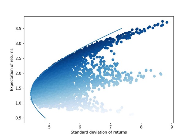
We can visualize the efficient in two ways. First, we can visualize many random portfolio by drawing random weights,

$$ \begin{equation} \textbf{w}\overset{\text{iid}}{\sim}\text{Dirichlet}(\alpha), \end{equation} $$

and then computing each portfolio’s $(x,y)$-coordinates of the portfolio using the equations for $\mu_p$ and $\sigma_p$. We can see the efficient frontier as the implicit parabolic edge.

We can optimize MPT to numerically approimate the weights $\text{w}$ for a variety of returns (sweeping the $y$-axis) for a fixed $K$. This produces the red line in the next figure. Here we generate $5,000$ random portfolios, generated by drawing weights $\textbf{w}$ from a Dirichlet distribution hyperparamters $\alpha=[1,1,1,1,1]$. The red line is the efficient frontier, approximated using constrained optimization.

The return of each portfolio is defined by the Sharpe Ratio, which is

$$ \text{Sharpe ratio}\overset{\Delta}{=}\frac{\mu_p-r_f}{\sigma_p} $$

where $r_f$ is the risk-free rate, a return that is assumed to be achievable without any risk. The Sharpe ratio is also related to other important ideas in portfolio theory, such as the tangent portfolio.

Investors also need to take note of the portfolio’s alpha, which is a measure of a portfolio’s risk-adjusted performance. There isn’t really a formal mathematical definition of alpha, but most people generally refer to Jensen’s alpha, which is

$$ \overset{\text{Jensen's alpha}}{\alpha_J}=\overset{\text{portfolio return}}{R_i}-[\overset{\text{risk free rate}}{R_f}+\overset{\text{portfolio beta}}{\beta_{iM}}\cdot(\overset{\text{market return}}{R_M}-\overset{\text{risk free rate}}{R_j})] $$

Limits of diversification

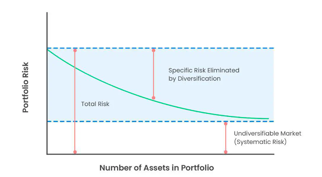
As we have seen, uncorrelated assets allow us to reduce a portfolio’s overall volatility. The ups and downs are less volatile. However, you can only achieve so much benefit by adding more assets to a portfolio. Think of it as the “Laws of Diminishing Returns.” We can see that as the number of assets in the portfolio increases, the portfolio variance decreases.

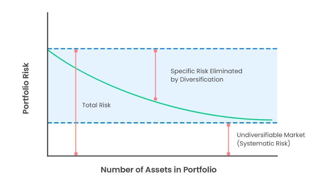
However, notice the benefits of diversification are constrained not only by the portfolio variance, but what we call “systematic risk”. In essence, investors aren’t compensated for taking what we call “unsystematic risk,” that is, risk that can be diversified away. Recall that the Equity Risk Premium is denoted by $E[r]=r_\alpha-r_f=\beta_\alpha(r_m-r_f)+\epsilon$.

Looking at the derivation of the Capital Asset Pricing Model (CAPM), we should receive a premium for investing in equities over debt, particularly the risk-free rate ($r_\alpha-r_f$). This makes sense, as without this premium, there would be nothing to entice owners of capital to invest in equities over treasuries. Also, investors should expect a premium for the systemic risk of the overall market $\big(\beta*(r_m-r_f)\big)$. Since equities are significantly more risky than treasuries, and given the universe of stocks has $\beta>1$ (meaning, most stocks are positively correlated), it is nearly impossible to diversify away systemic risk.

Conclusion

According to Modern Portfolio Theory, diversification reduces risk because uncorrelated assets reduce the portfolio’s overall volatility. The covariance between different assets is more critical than the variance of individual assets. However, portfolios are limited by diminishing returns and systematic risk. Overall, investors should seek to construct portfolios somewhere on the efficiency frontier since these portfolios have better risk-adjusted returns or more significant Sharpe ratios than portfolios inside the frontier.

[1] Markowitz, H. (1952) Portfolio selection. Journal of Finance.

[2] Markowitz, H. (1955) The optimization of a quadratic function subject to linear constraints.

[3] Sharpe W. F. (1966) Mutual Fund Performance. The Journal of Business, 39(1), 119-138

[4] Fidelity Investments (2024) Why diversification matters.