Revisitng Delta

I’ve recently been tasked with working more with more fixed-income derivatives, so I’m writing this more as a refresher for myself, but I’ve always guaged how well I know something based on how well I’m able to teach others.

Recall that the Black-Scholes price of a European-style call option is

$$ \begin{equation} \begin{aligned} C & = S\Phi(d_1)-Ke^{-rT}\Phi(d_2),\ d_1 & = \frac{1}{\sigma\sqrt{T}}[log(S/K)+[r+(1/2)\sigma^2]T],\ d_2 & = d_1-\sigma\sqrt{T}, \end{aligned} \end{equation} $$

where $\Phi(x)$ is the cumulative distribution function (CDF) of the standard normal distribution:

$$ \begin{equation} \begin{aligned} \Phi(x):=\frac{1}{\sqrt{\pi}}\int^{x}_{-\infty}e^{-z^2/2}dz \end{aligned} \end{equation} $$

Since $\Phi(x)$ is the CDF of the standard normal distribution, its derivation $\Phi^\prime(x)$ is the probability density function(PDF) of the standard normal distribution. I’ll denote this with $\phi(x)$ or

$$ \begin{equation} \phi(x):=\Phi^{\prime}(x). \end{equation} $$

Delta ($\Delta$) captures the sensitivity, or more precisely the instanteneous rate of change, of the option price to the spot price. The Black-Scholes delta for a call option is

$$ \begin{equation} \Delta(C)=\frac{\partial C}{\partial S}=\Phi(d_1) \end{equation} $$

where $\Phi(x)$ and $d_1$ are defined in Equations 1 and 2.

To understand delta, let’s start with an example. Suppose we have a stock with a price of $S=100$, a call option with a price of $C=10$, and a delta between the two of 0.7. (The prices do not matter here but will be in later examples.) Now imagine that we sell calls for $3000$ shares of this stock and want to hedge our resulting short position. We can use delta to compute the appropriate size of our hedge. We should put $0.7\times 3000=2100$ shares of the underlying stock. Why? This is just a direct application of Equation 4.

First, let’s replace the differentials (e.g., $\partial C$) with small moves in the asset (e.g., $dC$). This is a fine thing to do because Equation 8 says that $\Delta$ is the linear appropriate of how the Black-Scholes prices of our calls will change. We can write this as

$$ \begin{equation} \begin{aligned} dC=\Delta\times dS. \end{aligned} \end{equation} $$

Now let $w$ denote the number of shares of the stock assoicated with the calls we sold (here $w=3000$). Then by equation 5, we have

$$ \begin{equation} dC\times w = \Delta \times dS \times w \end{equation} $$

Our proposed hedge above is $\Delta \times w = 2100$, and this works because if the stock price changes by $dS=1$, then the call moves by $dC=0.7$, and we will make $2,100$ on our hedge and lose $0.7\times 3000=21000$ on our calls. In practice, this calculation is slightly more tedious because options are typically sold with a contract multiplier indicating the number of shares per contract, but this is just a matter of bookkeeping.

Thus, while the options we have sold have a delta of $0.7$, our actual portfolio position has a zero delta. We say that our portfolio is delta neutral, which means that if the spot changes a little, the value of our options position does not change significantly.

Dollar Delta

In the previous example, the raw values of the stock and call did not matter, and we had no sense of our total notional exposure. Thus, in practice, mathematical delta (Equation 4) is often converted to dollar delta, sometimes called notional delta, because this quantity tells us how much notional exposure we have to the underlying. A dollar delta is just delta times the spot price or

$$ \begin{equation} $\Delta=\Delta S \end{equation} $$

For example, our notional exposure in the previous example was the number of shares times dollar delta or

$$ \begin{equation} \begin{aligned} $\Delta\times w & = \Delta\times S\times w \ & = 0.7\times$ 100\times 3000 \ & = $ 210,000. \ \end{aligned} \end{equation} $$

To hedge, we should buy $210,000$ of stock, which is obviously the same as buying $2,100$ shares of stock at $S=100$.

One benefit of considering a notional amount is that we can multiply the dollar delta by a percent change in the stock. In contrast, since delta represents a dollar change in stock move, per dollar change in option move, we cannot directly multiply mathematical delta by a relative move such as a return or percent return. To see this, consider the returns in our running example. Let $S_1$ denote the stock price after moving $dS$. Then, the return on $S$ is

$$ \begin{equation} R_S=\frac{s_1-S}{S}=\frac{101-100}{100}=0.01 \end{equation} $$

while the return on C to a new price $C_1$ is

$$ \begin{equation} R_C=\frac{C_1-C}{C}=\frac{\Delta dS}{C}=\frac{0.7}{10}-0.07 \end{equation} $$

And clearly

$$ \begin{equation} \Delta R_S=0.7\times 0.01=0.007\neq 0.07=R_C \end{equation} $$

So, multiplying the mathematical delta by a relative move is nonsensical. Given Equation 8, we must operate on it in a way that makes sense.

However, we can multiply dollar delta by a relative move since

$$ \begin{equation} \begin{aligned} $\Delta\times R_S &= \Delta\times S\times\bigg(\frac{S_1-S}{S}\bigg)\ &= \Delta\times dS \ &= dC. \end{aligned} \end{equation} $$

The dollar delta is nice because it tells us our notional exposure to the underlying and because we can multiply it by a relative move in the underlying to get a dollar change in the option.

Portfolio Delta

Imagine we had a portfolio of $n$ options. We can represent the value of our portfolio, $V_p$, as a weighted sum of these $n$ assets,

$$ \begin{equation} V_p=\sum_{i=1}^nw_i V_i, \end{equation} $$

where the portfolio weights represent the quantity of each option, and where $V_i$ is the value of the $i$-th call or put. By the linearity of differentiation, we can efficiently compute the delta of this portfolio.

$$ \begin{equation} \begin{aligned} \Delta(V_p) &= \frac{\partial V_p}{\partial S} \ &= \sum_{i=1}^{n}w_i\frac{\partial V_i}{\partial S} \ &= \sum_{i=1}^{n}w_i\Delta(V_i) \end{aligned} \end{equation} $$

Thus, the delta of a portfolio can be computed by adding up the deltas of the individual options.

For example, recall our short position in call options from the example above. Now imagine that we additionally have a long position in call options worth 2000 shares of the same underlying, where the delta of each option is $0.6$. The delta of our portfolio in shares of stock is

$$ \begin{equation} \begin{aligned} -3000(0.7)+2000(0.6) &= -2100+1200\ &=-900. \end{aligned} \end{equation} $$

Thus, our portfolio has a dollar delta of—$90,000$, which we can make delta-neutral by buying $90,000$ of stock. This makes sense. Before, we had a notional hedge of $210,000$. Now, given our long position in calls that behave roughly like half a stock, we have a notional hedge that is roughly half that.

Delta Hedging

In our leading example, we hedged our delta from our option position, a short position in calls. Now that we understand the dollar delta, let’s think about a more general way to formulate the problem. Imagine a portfolio with a $\delta_{\Pi}$ delta. And imagine that another asset has a delta of $\Delta_i$. Then, to be delta neutral, we want to buy $w_i$ of this asset such that

$$ \begin{equation} w_i+\Delta_{\Pi}=0 \end{equation} $$

Solving for $w_i$, we get

$$ \begin{equation} w_i=-\frac{\Delta_{\Pi}}{\Delta_i} \end{equation} $$

But what asset should we use here? We could find an option with a delta of $\Delta_i$, but a more straightforward thing would be to buy the underlying asset, which has a delta of one $(\Delta_i=1)$. So, our hedge in shares or dollars should be proportional to $w_i=\Delta_{\Pi}$, which is what we see in Equation 10. We can easily consider this regarding shares or dollars by multiplying both sides of Equation 21 as desired.

Functional Form

Now that we understand how delta is used let’s dig into the precise definition of the Black-Scholes delta (Equation 8). This is an interesting result, but what it means may take time to be noticeable. First, note that since $\Phi(x)$ is the CDF of symmetric distribution, we can immediately guess that the delta’s shape is roughly a sigmoid function, which it is. This also makes sense if we visualize the slope of the tangent line changing as we move along the Black-Scholes price curve.

The delta for a call must initially be nearly zero when $S \ll K$, increase as $S$ approaches and passes $K$, and finally flatten off to almost one when $S\gg K$.

Notice that an at-the-money (ATM) option has a delta of slightly greater than 0.5. This is because while $\Phi(x)$ is symmetric with respect to its input $d_1$, the variable $d_1$ is a logarithmic function of $S$. Confusingly, some people will claim that the delta of an ATM option is 0.5. For example, Investopedia says

An ATM option as a delta of $\pm 0.50$, positive if it is a call, negative for a put.

But this is false. Just consider the full definition of delta for a call when $S=K$.

$$ \begin{equation} \Delta(C)=\Phi\bigg(\frac{[r+(1/2)\sigma^2]\sqrt{T}}{\sigma}\bigg). \end{equation} $$

since $\phi(x)$ is the cdf of the standard normal distribution, we can see that $\delta(c)=0.5$ only when $t=0$, assuming interest rates and volatility are nonzero. However, it only makes sense to talk about the delta of an atm option at expiry. We’ll discuss this when we discuss delta sensitivities to other parameters.

In most realistic scenarios (positive interest rates, nonzero volatility, and nonzero time expiry), the term $d_1$ is greater than zero when $S=K$, and thus the Black-Scholes delta of an ATM option is slightly greater than $0.5$.

A deep-in-the-money (ITM) option has a delta close to one, meaning it behaves like the spot. A deep out-of-the-money (OTM) option has a delta close to zero, meaning it is insensitive to the underlying price changes. Many of these points should hold for any option pricing model. However, it does not make sense to have an option pricing model with zero delta for an ITM option. So, the coherence of Black-Scholes Greeks with reality justifies this model.

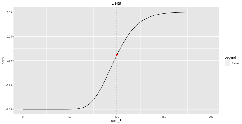
It makes sense that the delta for a call option is in the $[0,1]$ since $\Delta$ is the slope of the relationship between the spot and option. Using put-call parity, we can immediately derive the delta for a put:

$$ \begin{equation} \begin{aligned} \Delta(P) &= \frac{\partial}{\partial S}P \ &= \frac{\partial}{\partial S}(C+Ke^{-rT}-S) \ &= \Delta(C)-1. \end{aligned} \end{equation} $$

Since $\Delta(C)$ ranges in $[0,1]$, clearly $\Delta(P)$ is in the range [-1,0]. And this makes sense, given the Black-Scholes price curve for a put (figure 2). So the delta for a call and put have the same shape for all input parameters but are shifted by one.

Moneyness

At this point, we have enough understanding of delta to investigate a common interpretation of it: that it captures an option’s moneyness and how likely it is that the option ends ITM.

To understand this, we need to understand $\Phi(d_1)$ and $\Phi(d_2)$ from the Black-Scholes equation. $\Phi(d_2)$ has a clean interpretation. It is the probability that the option ends ITM in a risk-neutral world. If this is unclear, interpret $\Phi(d_2)$ by mapping it onto the appropriate term in the binomial options-pricing formula, a discrete-time analog of Black-Scholes.

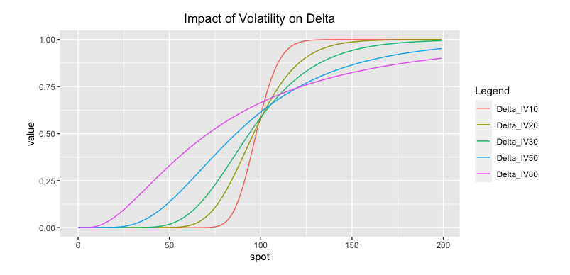
But since the moneyness interpretation of $\Phi(d_2)$ is accurate, it is only true of $\Phi(d_1)$ to the extent that $d_1\approx d_2$. How are these terms different? They differ by the volatility of the spot:

$$ \begin{equation} d_2=d_1-\sigma\sqrt{T} \end{equation} $$

This reasoning suggests that the moneyness interpretation of delta is approximately accurate when volatility or time to expiry is low but is less accurate when volatility or time to expiry is high. This is precisely the relationship we see when we compare $\Phi(d_1)$ and $\Phi(d_2)$ for varying volatilities.

Delta Sensitivity

As we have seen already, the precise shape of the delta changes based on the other Black-Scholes inputs. Just as we can understand Black-Scholes by fixing all parameters but one, we can understand a single Greek, such as delta, by fixing all other parameters.

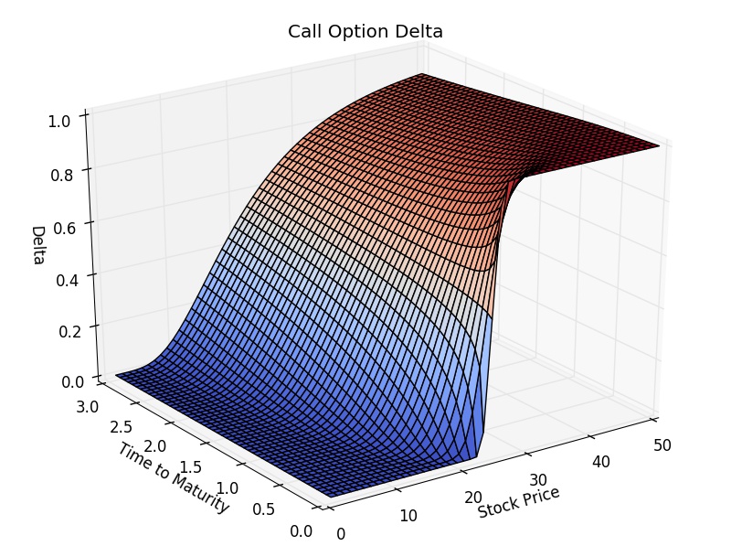
First, let’s look at how delta changes while holding all other parameters fixed as the time to expiry $T$ decreases. I like plotting this with $T$ decreasing since the graph can be read left to right as physical time progresses. We can see that all options, regardless of money, have more similar deltas when the expiration date is far enough out. Then, as expiration approaches, ITM, ATM, and OTM options cover the delta of $1$, $0.5$, and $0$, respectively, for calls and $0$, $-0.5$, and $-1$, respectively, for puts.

Another way to see this is to visualize how the Black-Scholes price curve (for calls) changes as a function of time. In the left subplot of Figure 2, I plotted the Black-Scholes price curve for a call as the time to expiry $T$ decreases to zero. As we can see, when $T$ is large, the option’s delta is roughly 0.5 over an extensive range of stock values.

Changing Delta

Finally, it is essential to remember that delta is a derivative and is, therefore, the slope of the tangent line to the Black-Scholes price curve at a particular spot price! When the spot changes in value from $S$ to $S_1$, our original estimate of the delta is no longer correct. It should be a new value $\Delta_1$, representing the slope of the line tangent to the Black-Scholes price curve at $S_1$.

Hedging an options position by trading the underlying requires continuously rebalancing the hedged position due to this continuously accumulating hedging error. One way to visualize this ever-changing error is by visualizing the gap between the linear equation $\Delta S_1+b$ and $\Delta_1 S_1+b_1$, where $b$ and $b_1$ and the $y$-intercepts their respective delta. What would increase this gap between the two points? More curvature to the Black-Scholes price curve.

This, in order to account for this hedging error, we could add a term that accounts for the curvature of the Black-Schole’s model a particular point. To do this, we use a second-order Greek called gamma, which we will get into in another post.

References

[1] Daniel Sevcovic, Beata Stehlikova, Karol Mikula (2011). “Analytical and numerical methods for pricing financial derivatives”. Nova Science Pub Inc; UK.

[2] Wilmott Paul (1994), “Option pricing - Mathematical models and computation”. Oxford Financial Press.

[3] Steven Shreve (2005), “Stochastic calculus for finance”. Spring Finance

[4] Paul Wilmott (2006), Paul Wilmott on quantitiative finance

[5] Broadie, Glasserman, Kou. Connecting Discrete and Continuous Path-Dependent Options