Measuring Pandemic Progress: Log Scale vs. Per Capita

Apr 15, 2020 3 min read Data Science, Programming, Statistics

There have been many visualization projects created for the purposes of modeling COVID-19 cases and deaths. The best known are the graphs produced by John Burn-Murdock of the Financial Times. You can view his very create and beautiful COVID visualizations on his Twitter Page.

Before COVID, I think people were more used to viewing data in relative terms. Now, log-scale visualizations have become more widespread, primarily due to the way diseases spread during a pandemic.

It's become so popular, programmers developed ways to replicate these charts using Python and R packages. The most notable being tidycovid19 package designed by Joachim Gassen. You can few the package on his GitHub [1].

# Importing all of the necessary packages
library(tidyverse)
library(tsibble)
library(tidycovid19)

# selecting how the data will be formatted
updates <- download_merged_data(cached = TRUE)

# plotting the countries of interests, 
countries <- c("AUS", "NZL", "ITA", "ESP", "USA", "GBR")

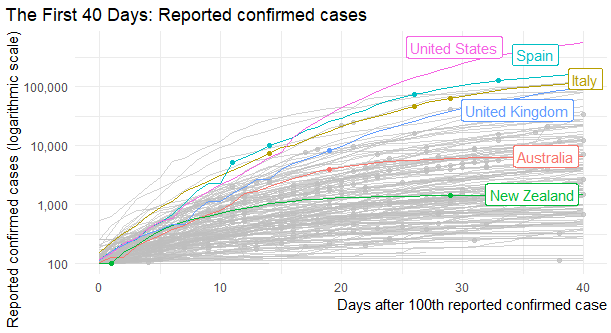
updates %>%
  plot_covid19_spread(
    highlight = countries,
    type = "confirmed",
    edate_cutoff = 40,
    min_cases = 100
  )

However, people have often wondered why we don't present these numbers on a per capita basis? Burn-Murdock has provided a data-oriented reason why log-scales are used instead of per capita scaling.

It isn't always clear when per capita metrics should (or should not) be used. However, many don't often realize how per capita figures can distort the story of what is going on in the region.

For example, Switzerland has 2,975 cases per capita, while the United States has 1,841 cases per capita [2]. However, cases are currently growing and doubling faster in the U.S. compared to Switzerland [3]. Obviously, Switerzland's high per capita figure is primarily attributed to its small population size, not its response to containing the virus.

Simply put: per capita figures makes small countries look big, and vice versa. Not only that, per capita figures only shifts the curves vertically; it would not change the trajectory or slope of the curves. Remember the following:

\[log(Y_{t}/P_{t})=log(Y_{t})-log(P_{t})\]

Where $Y_{t}$ is the number of cases on dat $t$ and $P_{t}$ is the population on day $t$. Population doesn't change much over a period of time, so per capita figures involves subtracking a constant from the log case data.

The same point applies to the differences in testing policies between countries. If Country A is testing more as a percentage of the population relative to Country B, then these differences will show up as a vertical difference between the plots. They won't; however, show up in the trajectory.

Although these choices are still a bit of a judgment call (not standard among statisticians), we should look at the slope of the lines if we want to explore how countries are responding to the pandemic relative to others.

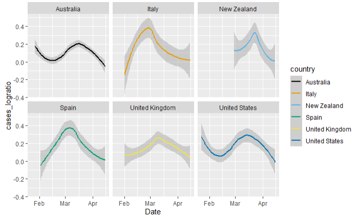
While the graph doesn't tell us everything about how the pandemic is overwhelming the different health care systems around the world, it does show how each country is attempting to slow the infection rate and reduce the slope of their curves. It's easier to compare the trajectory in this way, considering that we have to look to see which country is trending higher.