The Mathematics of Pandemics
So, this is our very first pandemic. At least, it’s the first serious pandemic. I’ve lived through the 2009 H1N1 Pandemic, but I don’t really remember it all that well. All I know is that H1N1 is not nearly as serious as this, because now I’m forced to work from home.
Right now, COVID-19, a.k.a, the coronavirus is on our doorstep. There are more than 423,000 confirmed cases in the United States; 14,700 confirmed deaths [1]. New York has the highest record death toll; we surpassed Washington State a few weeks ago. It certainly does feel like an apocalyptic scenario is about to occur.
Regardless, one good thing that can occur out of this situation is that the Coronavirus has rekindled the public’s interest in Mathematics. At least, marginally. Articles are circulating explaining “dangerous mathematics behind the coronavirus,” and how cases could grow exponentially [2].
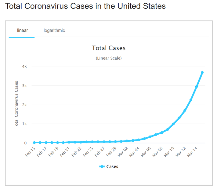
The idea behind exponential growth as it relates to pandemics is that one person who has contracted the virus comes into contact with anyone. So the total number of cases increases to 2. Assume each infected person will come in contact with 1 new person. Then those 2 infected people will infect 2 more people, increasing confirmed cases to 4. Those 4 will eventually become 8, then 8 becomes 16, and so on.
This is how COVID-19 could work, but at best, it’s an oversimplification. Everyone online (and by everyone, I mean Twitter) has an opinion on what they believe will happen. Some people are behaving like it’s the end of the world; others think this will be over by Easter.
I, on the other hand, found that it is more useful to learn about the methodologies epidemiologists are using the model the virus.
The SIR Model
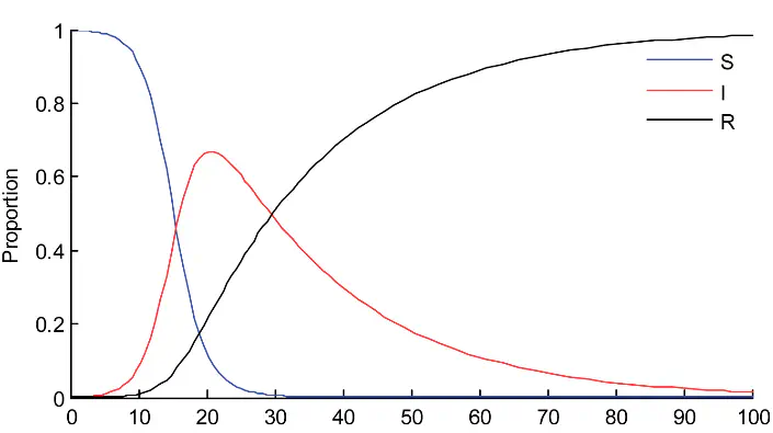
The SIR model is a simple model developed by Ronald Ross and William Hamar, but greatly expanded by Anderson McKendrick and William Kermack, which simplified the process. Using this model, we assume the population consist of three types of individuals, which are denoted by variables $S$, $I$, and $R$.
- $S$ is the number of susceptibles; who are not infected, but could become infected at a later point.
- $I$ is the number of infectives; individuals who have the diease and can transmit to others.
- $R$ is the number of recovered or removed; they cannot become infected or transmit to others.
It should be noted that people that have recovered from a virus may have developed a natural immunity over time, or they may have currently been in isolation, or they may have died. The SIR model doesn’t distinguish between these possibilities.
New infections will occur as a result of contact between infectives and susceptibles. In the SIR model, the rate at which new infections happen (as a function fo time) is $\beta$, $S$, $I$, for some positive constant $\beta$. These interactions occur as a form of “mixing,” and mixing allows us to utilize ordinary differential equations (ODE).
You don’t need any knowledge about differential equations. However, derivatives are how mathematicians describe the rate of change of as time goes on.
$$ \begin{aligned} \frac{dS}{dt} & = -\beta \cdot S \cdot I \ \frac{dI}{dt} & = \beta \cdot I \cdot \frac{S}{N} - \nu \cdot I \ \frac{dR}{dt} & = \nu \cdot I, \end{aligned} $$
where the diease transmission rate $\beta > 0$, and the recovery rate $\nu > 0$ (or in other words, the duration of infection $D=1/\nu$).
As you may have noticed, that total population $S+I+R$ is constant because the differential equation $\frac{dS}{dt}+\frac{dI}{dt}+\frac{dR}{dt}=-\beta IS+(\beta IS -\nu I) + \nu I=0$
It’s probably easier to visualize this instead of talking about this subject in the abstract. There are some developers on GitHub that have implemented the SIR model for creating an infectious disease model. One of whom goes by the name of Henri Froese, who is a computer science student [3].
Model Parameters
We want to derive our differential equation, $\frac{dS}{dt}$, $\frac{dI}{dt}$, and $\frac{dR}{dt}$ with the parameters $S$, $I$, $R$, $\beta$, and $\nu$. We will also adjust for the population
# creating a function for the differential equation
def deriv(y, t, N, beta, nu):
    S, I, R, = y
    dSdt = -beta * S * I / N
    dIdt = beta * S * I / N - nu * I
    dRdt = nu * I
    return dSdt, dIdt, dRdt
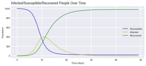
We’re simulating a pandemic in a town with a population of 1,000 (not a very large but it’s easier to wrap your head around). We will assume that an infected person infects one other person per day ($\beta = 1$).
For our made up virus, we will set the duration of infection for four days. The initial condition starts with one infection, which leaves 999 susceptible people (and no recoveries, so far).
N = 1000
beta = 1.0
D = 4.0
nu = 1.0 / D
S0, I0, R0 = 999, 1, 0

t = np.linspace(0, 49, 50)
y0 = S0, I0, R0
ret = odeint(deriv, y0, t, args=(N, beta, nu))
S, I, R = ret.T
The solution to a differential equation is any condition that satisfies it, so we are going to use the odeint method to integrate the differential equation. Afterward, we unpack the results for S, I, and R into variables which we can then plot.
The Diease Always Dies Out
There are lots of high profile individuals; particularly, President Trump has suggested that the virus will go away on its own without a vaccine [4]. This may happen; it may not happen. We don’t know enough about the virus to determine if this is true. One thing is certain; we know enough about the epidemiology to say that the virus disappearing isn’t outside the realm of possibility [5]. Mathematically, we can prove this by contradiction.
Consider the differential equation for the recovery rate, $\frac{dR}{dt}=\nu I$. Let’s say that the initial condition $I(\infty)=0$ for all initial conditions, without having a formula for $I(t)$. If not, $\frac{dR}{dt}=\nu I$ implies that for $t$ sufficiently large, $\frac{dR}{dt}>\nu I(\infty)/2>0$, and this implies that $R(\infty)=\infty$, which is a contradiction.
As such, at some point, the virus will eventually die out. It’s all a matter of how many people must become infected with the virus.
The Epidemic Threshold Theorem
The effective reproductive number $R_{e}=(S(0)/N)b/\nu$ and the basic reproductive number $R_{0}=b/\nu$. If the entire population is initially susceptible, for example, $S(0)=N-1, I(0)=1, R(0)=0,$ and large (the model’s assumption), then $R_{e}=((N-1)/N)b/\nu$ is approximately equal to $R_{0}$. As such, we will assume the quantity $(N-1)/N$ is equal to 1.
As we can see in our simple model, confirmed cases peak around day 10 and addition cases begin to decrease until the virus finally dies out. We already observed that $(\frac{dI}{dt})(0)=\nu (R_{e}-1)I(0)$, which implies that the number of infected individual initially starts growing/decreasing exponential at the rate $\nu(R_{e}-1).$
As such, there are two conditions that determines whether an infectious diease will quickly die out or whether it will invade the population can cause an epidemic:
- Case #1: If $R_{e}\leq 1$, then $I(t)$ decreases monotonically to zero as $t \rightarrow \infty $.
- Case #2: If $R_{e}\geq 1$, then $I(t)$ starts increasing, reaches its maximum, and then decreases to zero as $t \rightarrow \infty$. The scenario of the increasing number cases is what starts an epidemic.
We will plot how this works using Python.
def plotsir(t, S, I, R):
    f, ax = plt.subplots(1, 1, figsize=(10, 4))
    ax.plot(t, S, 'b', alpha=0.7, linewidth=2, label='Susceptible')
    ax.plot(t, I, 'y', alpha=0.7, linewidth=2, label='Infected')
    ax.plot(t, R, 'g', alpha=0.7, linewidth=2, label='Recovered')

    ax.set_xlabel('Time (days)')

    ax.set_title(
        'Infected/Susceptible/Recovered People Over Time', fontsize=14, x=.27, y= 1.01)
    ax.yaxis.set_tick_params(length=0)
    ax.xaxis.set_tick_params(length=0)
    ax.grid(b=True, which='major', c='w', lw=2, ls='-')
    legend = ax.legend()
    legend.get_frame().set_alpha(0.5)
    for spine in ('top', 'right', 'bottom', 'left'):
        ax.spines[spine].set_visible(False)
    plt.show()

plotsir(t, S, I, R)
Here is the output of the model.
The SEIR/SEID Model
The first SIR model is much too simple for our very complicated situation. We also may need to consider the fact that people who have the virus may not exhibit any symptoms. Some people who contract a virus may not immediately become infectious, at least, not to the point where they spread the virus around to other people. This period is known as the incubation period. The incubation period is the time between the exposure of a disease when symptoms of the disease begin to show.
Right now, we estimate that the incubation period for COVID-19 is a little over 5 days. The vast majority of people who begin to show symptoms usually do so within 11.5 days of infection [6]. However, the problem with the incubation period with COVID-19 is that people become infectious without showing any symptoms at all. These factors are what makes the coronavirus particularly deadly.
Because of the complexity of the incubation period, we need to account for another variable, the Exposed. As such, we introduce the variant of the SEIR model: Susceptible people contract the virus, then become exposed, then become infected, then eventually recover. We introduce a new variable to represent the rate at which those exposed become infected, $\delta$.
We also need to account for the fact that some people never recover from the virus. Some people pass away due to complications related to a disease, as it is the case with COVID-19. Of course, you can only die from a disease that you’ve been exposed to, so we introduce a new variable, $\rho$, which represents the rate at which people die from the virus.
Considering we have two possibilities, recovery and death, we need to account for the probability of going from infected to recovered or dead. We introduce one more variable, $\alpha$, which accounts for the death rate. Suppose 100 people are infected a day; 5% are estimated to die from the virus. Given these factors, 95% of people are estimated to recover.
The probability of going from infected to death is $alpha$ and the probability of going to from infected to recovered is $1-\alpha$.
As such, we have the following differential equations:
$$ \begin{aligned} \frac{dS}{dt} & = -\beta \cdot I \cdot \frac{S}{N} \ \frac{dE}{dt} & = \beta \cdot I \cdot \frac{S}{N} - \delta \cdot E \ \frac{dI}{dt} & = \delta \cdot E - (1-\alpha) \cdot \nu \cdot I - \alpha \cdot \rho \cdot I \ \frac{dR}{dt} & = (1 - \alpha) \cdot \nu \cdot I \ \frac{dD}{dt} & = \alpha \cdot \rho \cdot I \end{aligned} $$
New Model Parameters
We want to derive our differential equation, $\frac{dS}{dt}$, $\frac{dE}{dt}$, $\frac{dI}{dt}$, $\frac{dR}{dt}$ and $\frac{dD}{dt}$ with the parameters $S$, $E$, $I$, $R$, $\alpha$, $\beta$, $\delta$, $\rho$, and $\nu$. We will also adjust for the population.
def deriv(y, t, N, beta, nu, delta, alpha, rho):
    S, E, I, R, D = y
    dSdt = -beta * S * I / N
    dEdt = beta * S * I / N - delta * E
    dIdt = delta * E - (1 - alpha) * nu * I -alpha * rho * I
    dRdt = (1 - alpha) * nu * I
    dDdt = alpha * rho * I
    return dSdt, dEdt, dIdt, dRdt, dDdt
This time, we’re going to use a town with the population of 100,000 people. We will set the rate of exposure, or the incubation period ($\delta$), to five days. We’ll keep the duration of infection at 4 days. We will assume that the death rate from our virus is ~10%; and people generally die from the virus 9 days after infection.
def deriv(y, t, N, beta, nu, delta, alpha, rho):
    S, E, I, R, D = y
    dSdt = -beta * S * I / N
    dEdt = beta * S * I / N - delta * E
    dIdt = delta * E - (1 - alpha) * nu * I -alpha * rho * I
    dRdt = (1 - alpha) * nu * I
    dDdt = alpha * rho * I
    return dSdt, dEdt, dIdt, dRdt, dDdt

N = 100000
D = 4.0
nu = 1.0 / D
delta = 1.0 / 5.0
R_0 = 5.0
beta = R_0 * nu
alpha = 0.2
rho = 1/9
S0, E0, I0, R0, D0 = N-1, 1, 0, 0, 0

t = np.linspace(0, 100, 100)
y0 = S0, E0, I0, R0, D0
ret = odeint(deriv, y0, t, args=(N, beta, nu, delta, alpha, rho))
S, E, I, R, D = ret.T

plotseird(t, S, E, I, R, D)
The model provides the following output:
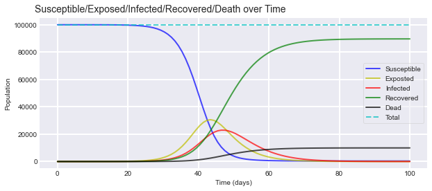
We added the total line to sanity check everything. All of the possible states should add up to 100,000. Based on the parameters, we could expect the virus to infect ~200,000 people while exposing ~350,000 people. The difference between the two comprises our asymptomatic cases. (people who have been exposed to the virus, but fail to show symptoms) Overall, the virus ends up killing ~100,000 people under our scenario.
Vaccination and Heard Immunity
There is a lot of talk about the potential for a vaccine, as well as this concept of herd immunity. Obviously, vaccinating susceptible individuals reduces the number of susceptible individuals. Even if the vaccine is 100% effective (for comparison, the flu vaccine is only ~60% effective), vaccinating an entire population is very expensive. Also, not everyone can take the vaccine.
We also need to consider the fact that some individuals have severe allergies or compromised immune systems; vaccines can be very critical [7]. Vaccinations alone aren’t enough to prevent (or end) an epidemic; it also requires a phenomenon called herd immunity.
Recall from before, to prevent an epidemic, $R_{e} \leq 1$. Let $\rho$ denote the fraction of the susceptible individuals who receieve a vaccination (assuming 100% effectiveness). These amount of vaccinated individuals ($\rho S(0)$) have moved from the susceptible class to the removed class. As such, the size of the susceptible class becomes $(1-\rho)S(0)$.
To prevent an epidemic, it is necessary that
$$(1-\rho) , S(0) ,\beta /\nu \leq 1$$
This will occur when $\rho \geq \rho_{c}$, where $\rho_{c}=1-1/R_{e}$ denotes the critical vaccination threshold.
When Will This Epidemic End?
No one knows for sure and right now we’re talking about staying locked down until the virus suddenly disappears (or until no one dies from it). This is probably not going to happen.
Consider what it would take to limit the number of susceptible individuals:
$$S(\infty) \geq S(0) , exp(-R_{0})>0$$
Dividing the differential equations for $dS$ and $dR$ yields the following ODE
$$\frac{dS}{dR}=\frac{-\beta IS}{\nu I}=\frac{-\beta S}{\nu}$$
This ODE is separable, since for $S>0$ it can be rewritten as
$$\int \frac{1}{S}dS=\int \frac{-\beta}{\nu}dR$$
Integrating both side yields
$$S(t) = S(0) , exp(-\beta (R(t)-R(0))/\nu)$$
Since $0 \leq R(t)-R(0)\leq N$ it follows that $S(t)\geq S(0), exp(-\beta N/\nu)$ and thus
$$S(\infty)\geq S(0), exp(-\beta N/\nu), =, S(0), exp(-R_{0})>0$$
As the epidemic continues, the number of susceptible individuals decreases, and so the rate at which new infections arise also decreases. Eventually, S(t) drops below $\nu/\beta$, and the rate at which individual recover exceeds the rate at which new infections occur. Thus, $I(t)$ starts decreasing.
The epidemic ends due to a lack of newly infected individuals, not because of the lack of susceptible individuals.
Source
[1] CBS News | Coronavirus updates from April 8, 2020
[2] Washington Post | Exponential growth of coronavirus offers perilous math in the context of coronavirus
[3] Henri Froese | Infectious Diease Modeling GitHub Repository
[4] Guardian News | Donald Trump says coronavirus will ‘go away without a vaccine’
[5] Brauer (2017) | Mathematical epidemiology: Past, present, and future
[6] University of Massachusetts Amherst (March, 2020) | Median incubation period for COVID-19
[7] Center for Diease Control | Weakened Immune System and Adult Vaccination
Andre Sealy
Quant Research / Data Scientist / Writer
My research interests involves Quantitative Finance, Mathematics, Data Science and Machine Learning.