Option Sensitivities, Formula Proofs, and Python Scripts: Part 1 (Delta)
The following is an general overview of vanilla options partial sensitivities (option greeks). This series will be a continuation of the project Option Payoffs, Black-Scholes, and the Greeks. We’ve already outlined the necessary terms for understanding Options and the Greeks here. In this post, I will be covering the first greek: Detla ($\Delta$).
The delta of an option, $\Delta$, is defined as the rate of change of the option price respected to the rate of change of the underlying asset price:
$$\Delta = \frac{\partial V}{\partial S}$$
As you know, $V$ is the value of the option while $S$ is the underlying asset price.
We’ve already covered the the Black-Scholes option pricing model for a call option on a non-dividend stock:
$$ C(S_{t},t) = N(d_{1})S_{t}-N(d_{2})Ke^{-r(T-t)} $$
With:
$d_{1} = \frac{1}{\sigma \sqrt{T-t}} \Big[ln\bigg(\frac{S_{t}}{k}\bigg)+\bigg(r+\frac{\sigma^{2}}{2}\bigg)(T-t) \Big]$
$d_{2} = d_{1} - \sigma \sqrt{T-t}$
However, we haven’t covered the Black-Scholes model for a put option, which is as follows:
$$P(S_{t},t)=-SN(-d_{1})+Ee^{-r(T-t)}N(-d_{2})$$
The call option Delta will be:
$$\Delta_{c}=\frac{dc}{dS}=e^{-qT}N(d_{1})$$
Proof
$$ \begin{aligned} \Delta_{c} = \frac{dc}{dS} & = \frac{d(e^{-qT}SN(d_{1})-Xe^{-rT}N(d_{2}))}{dS}\ & = e^{-qT}N(d_{1})+Se^{-qT}\frac{\partial N(d_{1})}{\partial S}-Xe^{-rT}\frac{\partial N(d_{2})}{\partial S} \ & = e^{-qT}N(d_{1})+Se^{-qT}\frac{\partial Nd_{1}}{\partial d_{1}}-Xe^{-rT}\frac{\partial d_{2}}{\partial S}\frac{\partial N(d_{2})}{\partial d_{2}} \ & = e^{-qT}N(d_{1})+Se^{-qT}\frac{\partial Nd_{1}}{\partial d_{1}}N^{\prime}(d_{1})-Xe^{-rT}\frac{\partial d_{2}}{\partial S}N^{\prime}(d_{2})\ & = e^{-qT}N(d_{1})+\underbrace{\frac{Se^{-qT}N^{\prime}(d_{1})}{S\sigma\sqrt{T}}-\frac{Xe^{-rT}N^{\prime}(d_{1})}{S\sigma\sqrt{T}}}_{I=0} \end{aligned} $$
Above, $I=0$. Referencing the equation for risk-adjusted lognormal probabilities, $d_{1}$, we have:
$$ \begin{aligned} ln(S/X&)+(r-q+\frac{\sigma^{2}}{2})T=d_{1}\sigma\sqrt{T} \ \implies & ln(S)-ln(X)+(r-q)T=d_{1}\sigma\sqrt{T}-\frac{\sigma^{2}}{2}T=\frac{1}{2}\big[d^{2}{1}-(d{1}-\sigma\sqrt{T})^{2}]\big] \ \implies & ln(S)+ln(\frac{1}{\sqrt{2\pi}})-\frac{d_{1}^{2}}{2}=ln(X)-(r-q)T+ln(\frac{1}{\sqrt{2\pi}})-\frac{d_{2}^{2}}{2} \ \implies & S\frac{1}{\sqrt{2\pi}}e^{-\frac{d_{1}^{2}}{2}}=Xe^{-(r-q)T}\frac{1}{\sqrt{2\pi}}e^{-\frac{d_{2}^{2}}{2}}\ \implies&SN^{\prime}(d_{1})=Xe^{-(r-q)T}N^{\prime}(d_{2})\ \implies&Se^{-qT}N^{\prime}(d_{1})=Xe^{-rT}N^{\prime}(d_{2}) \end{aligned} $$
From the derivation of $\Delta=\frac{dc}{dS}$, we obtain:
$$\Delta_{c}=e^{-qT}N(d_{1})$$
As we should have what is known as Call/Put Parity, we should have the following equation:
$$ \begin{aligned} p+S&e^{-qT}=c+Xe^{-rT}\ \implies&\frac{dp}{dS}=\frac{dc}{dS}-e^{-qT}\ \implies&\Delta_{p}=N(d_{1})-1 \end{aligned} $$
Here is the python script.
import numpy as np
from math import sqrt, pi, log, e
from enum import Enum
import scipy.stats as stat
from scipy.stats import norm
import time

class BSMerton:
    def __init__(self, args):
        # 1 for a Call, -1 for a put
        self.Type = int(args[0])
        self.S = float(args[1])                     # Underlying asset price
        self.K = float(args[2])                     # Option strike K
        self.r = float(args[3])                     # Continuous risk free rate
        self.q = float(args[4])                     # Dividend countinous rate
        self.T = float(args[5]) / 365.0             # Compute time to expiry
        self.sigma = float(args[6])                 # Compute time to expiry
        self.sigmaT = self.sigma * self.T ** 0.5    # sigma*T for reusability
        self.d1 = (log(self.S / self.K) +
                   (self.r - self.q + 0.5 * (self.sigma ** 2))
                   * self.T) / self.sigmaT
        self.d2 = self.d1 - self.sigmaT
        [self.Delta] = self.delta()

    def delta(self):
        dfq = e ** (-self.q * self.T)
        if self.Type == 1:
            return [dfq * norm.cdf(self.d1)]
        else:
            return [dfq * (norm.cdf(self.d1) - 1)]
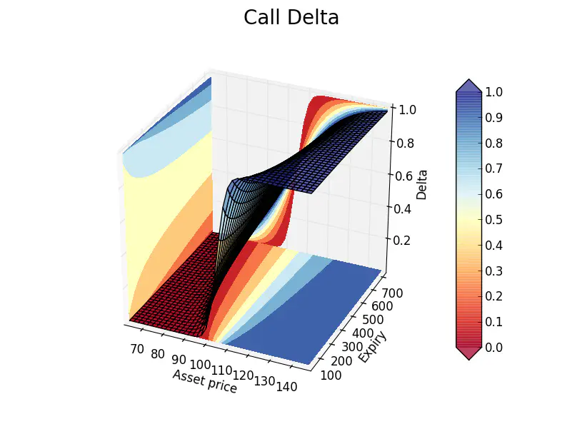
Code that you can use to calculate and chart Delta sensitivities.
import numpy as np
import matplotlib.pyplot as plt
from mpl_toolkits.mplot3d import Axes3D
import math
from matplotlib import cm
import OptionsAnalytics
from OptionsAnalytics import BSMerton

sigma = 0.12            # Flat volatility
strike = 105.0          # Fixed strike
epsilon = 0.4           # The % on the left/right of Strike.
# Asset prices are centered around Spot ("ATM Spot")
shortexpiry = 30        # Shortest expiry in days
longexpiry = 720        # Longest expiry in days
riskfree = 0.00         # Continous risk free rate
divrate = 0.00          # Continous div rate

# Grid deinition
dx, dy = 40, 40         # Step throughout asset price and expiries axis

# xx: Asset price axis, yy: expiry axis, zz: greek axis
xx, yy = np.meshgrid(np.linspace(strike*(1-epsilon), (1+epsilon)*strike, dx),
                     np.linspace(shortexpiry, longexpiry, dy))
print("Calculating greeks...")

zz = np.array([BSMerton([1, x, strike, riskfree, divrate, y, sigma]).Delta for
               x, y in zip(np.ravel(xx), np.ravel(yy))])

zz = zz.reshape(xx.shape)

Plot greek surface
print("Plotting surface...")
fig.subtitle('Call Delta', fontsize=20)
ax = fig.gca(projection='3d')
surf = ax.plot_surface(xx, yy, rstride=1, cstride=1,
                       alpha=0.75, cmap=cm.RdYlBu)
ax.set_xlabel('Asset price')
ax.set_ylabel('Expiry')
ax.set_zlabel('Delta')

# Plot 3D contour
zzlevels = np.linspace(zz.min(), zz.max(), num=8, endpoint=True)
xxlevels = np.linspace(xx.min(), xx.max(), num=8, endpoint=True)
yylevels = np.linspace(yy.min(), zz.max(), num=8, endpoint=True)

cset = ax.contourf(xx, yy, zz, zzlevels, zdir=’z’, offset=zz.min(),
                   cmap=cm.RdYlBu, linestyles=’dashed’)
cset = ax.contourf(xx, yy, zz, xxlevels, zdir=’x’, offset=xx.min(),
                   cmap=cm.RdYlBu, linestyles=’dashed’)
cset = ax.contourf(xx, yy, zz, yylevels, zdir=’y’, offset=yy.max(),
                   cmap=cm.RdYlBu, linestyles=’dashed’)

for c in cset.collections:
    c.set_dashes([(0, (2.0, 2.0))])  # Dash contours

plt.clabel(cset, fontsize=10, inline=1)

ax.set_xlim(xx.min(), xx.max())
ax.set_ylim(yy.min(), yy.max())
ax.set_zlim(zz.min(), zz.max())

# ax.relim() #ax.autoscale_view(True,True,True)

# Colorbar

colbar = plt.colorbar(surf, shrink=1.0, extend=’both’, aspect=10)
l, b, w, h = plt.gca().get_position().bounds
ll, bb, ww, hh = colbar.ax.get_position().bounds
colbar.ax.set_position([ll, b+0.1*h, ww, h*0.8])

# Show chart
plt.show()
Andre Sealy
Quant Research / Data Scientist / Writer
My research interests involves Quantitative Finance, Mathematics, Data Science and Machine Learning.